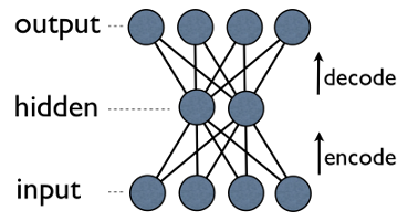
In this notebook, we look at how to implement an autoencoder in tensorflow. Autoencoders are a Neural Network (NN) architecture. The basic idea of an autoencoder is that when the data passes through the bottleneck, it is has to reduce. The result is a compression, or generalization of the input data.
This post is a nice summary for learning about the mechanics of autoencoders.
Starting off
As prerequisite, make sure tensorflow >1.0 is installed and TensorBoard ist started
tensorboard --logdir /tmp/tfboard
Tensorboard is a visualization utility for tensorflow that can be used to document the learning process of a NN. Tensorflow is a framework to define and run computational graphs. We use tensorflow to define the graph of an autoencoder in this notebook.
import tensorflow as tf
import numpy as np
import pandas as pd
import time
import pickle
import matplotlib.pyplot as plt
%matplotlib inline
from tensorflow.python.framework import ops

def movingaverage (values, window):
    '''Simple Moving Average low pass filter
    '''
    weights = np.repeat(1.0, window)/window
    sma = np.convolve(values, weights, 'valid')
    return sma

print(tf.__version__)
1.0.1
MultilayerPerceptron Class
To implement the autoencoder, we define a flexible class for feed-forward multilayer perceptron, a weird way of saying neural network. We use the term perceptrons loosely in this notebook. This class holds the code to define the NN and execute training and inference tasks. Moreover, it includes code to document the training process.
A NN is defined by the sizes and the activation function for each layer. These are two lists, layer sizes are integers, activation function can be arbitrary functions, common choices are tf.nn.relu between layers, or tf.nn.sigmoid for outputs.
Constructor
In its constructor, the starts off with some housekeeping and then defines the computational graph for the NN.
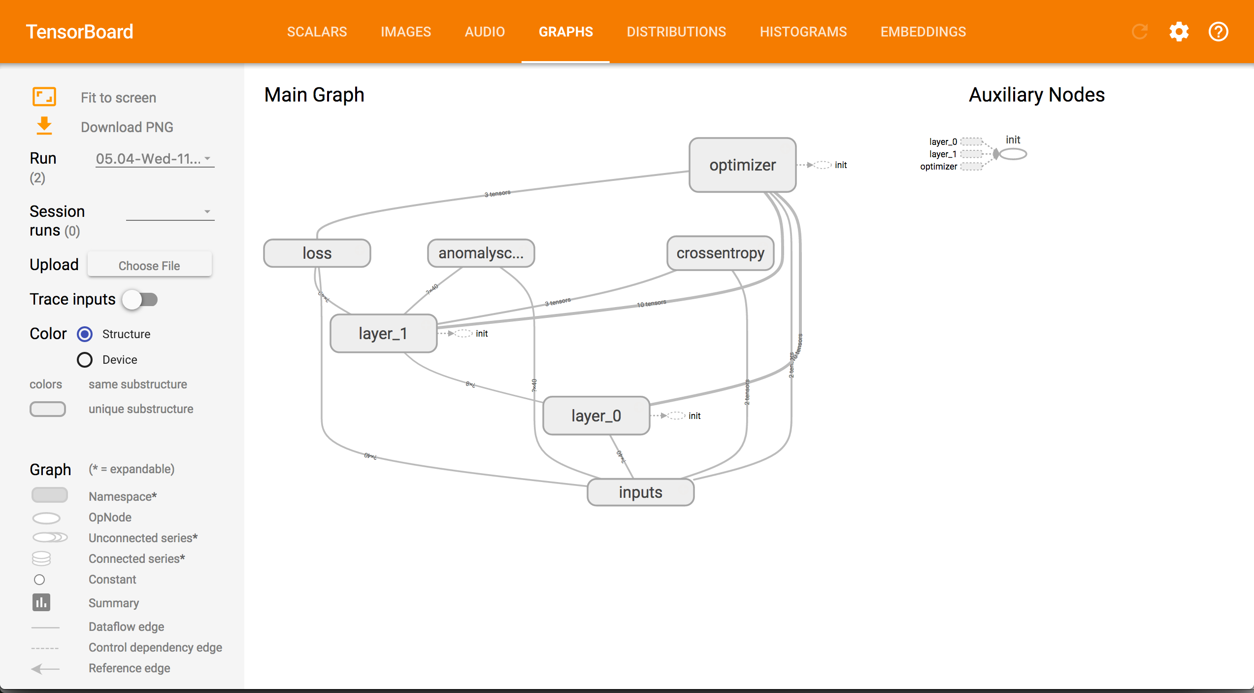
The NN’s inputs are specified as tf.placeholder that are replaced by the actual data during execution. The tf.name_scope command groups the inlined commands to make the graph better readable. It has no effect beyond documentation. The for loop defines the core of the NN. Each interation constructs a layer of perceptrons. The inputs of the current layer are connected to the previous layer. Inside a layer, we have the well known weights and biases that form a linear function: . Weights and biases are declared as tf.Variable , so that their values can change. The activation function adds non-linearity by squashing the output of the linear function in some particular range. For instance, the tf.nn.sigmoid function maps all input values to the interval . This graph constructed this way represents the structure of the NN.
A couple of other nodes in the graph define the operation of the NN. Most importantly, a loss/cost function defines how well the NN is achieving its goal. For instance, we use the mean-square-error in our class. This function is fed to the tf.train.AdamOptimizer (paper) that works to minimize the loss function. Note that the loss function is defined on the NN, thus the optimizer can access the NN’s graph as well. During execution, the optimizer changes the values of the tf.Variable in the graph of the loss function to minimize its output. The two functions anomalyscore and crossentropy can be used to evaluate the NN.
Finally, the variables are all initialized through a run call to the tf.Session, the log dir and it’s file writing facility are prepared.
Train method
When training, the optimizer adjusts the weights and biases in the NN in order to improve the NN. Most NNtraining is done using Stochastic Gradient Descent (SGD). SGD is interative and each training example is used to compute a small adjustment to weights and biases. In order to track the training process, we split the training dataset in smaller batches and measure the performance after training each batch. This performace record is logged locally and forwarded to tensorboard.
Predict method
Inference or prediction evaluates the NN graph for an input data set and outputs the classification result, or - in case of autoencoders - the reconstructed input.
Score method
A common way of computing anomaly scores in autoencoders is to use the reconstruction error of the NN. That is the difference of the inputs and the reconstructed outputs, reduced to a single number.
class MultilayerPerceptron:
    '''Class to define Multilayer Perceptron Neural Networks architectures such as
       Autoencoder in Tensorflow'''
    def __init__(self, layersize, activation, learning_rate=0.05, summaries_dir='/tmp/tfboard'):
        ''' Generate a multilayer perceptron network according to the specification and
            initialize the computational graph.'''
        assert(len(layersize)-1==len(activation),
		    'Activation function list must be one less than number of layers.')
        # Reset default graph
        ops.reset_default_graph()
        # Capture parameters
        self.learning_rate=learning_rate
        self.summaries_dir=summaries_dir+'/'+time.strftime('%d.%m-%a-%H:%M:%S',time.localtime())
        # Define the computation graph for an Autoencoder
        with tf.name_scope('inputs'):
            self.X = tf.placeholder("float", [None, layersize[0]])
        inputs = self.X
        # Iterate through specification to generate the multilayer perceptron network
        for i in range(len(layersize)-1):
            with tf.name_scope('layer_'+str(i)):
                n_input = layersize[i]
                n_hidden_layer = layersize[i+1]
                # Init weights and biases
                weights = tf.Variable(tf.random_normal([n_input, n_hidden_layer])*0.001,
				name='weights')
                biases  = tf.Variable(tf.random_normal([n_hidden_layer])*0.001, name='biases')
                # Create layer with weights, biases and given activation
                layer = tf.add(tf.matmul(inputs, weights), biases)
                tf.summary.histogram('pre-activation-'+activation[i].__name__, layer)
                layer = activation[i](layer)
                # Current outputs are the input for the next layer
                inputs = layer
                tf.summary.histogram('post-activation-'+activation[i].__name__, inputs)
        self.nn = layer
        # Define loss and optimizer
        with tf.name_scope('loss'):
            self.loss = tf.reduce_mean(tf.square(tf.subtract(self.nn, self.X)))
            tf.summary.scalar("training_loss", self.loss)
        with tf.name_scope('optimizer'):
            self.optimizer = tf.train.AdamOptimizer(
			learning_rate=self.learning_rate).minimize(self.loss)
        with tf.name_scope('anomalyscore'):
            self.anomalyscore = tf.reduce_mean(tf.abs(tf.subtract(self.nn, self.X)), 1)
        with tf.name_scope('crossentropy'):
            self.xentropy = tf.reduce_mean(tf.nn.softmax_cross_entropy_with_logits(
			                                        logits=self.nn, labels=self.X))
            tf.summary.scalar("cross_entropy", self.xentropy)
        # Init session
        init = tf.global_variables_initializer()
        self.sess = tf.Session()
        self.sess.run(init)
        # Configure logs
        tf.gfile.MakeDirs(summaries_dir)
        self.merged = tf.summary.merge_all()
        self.summary_writer = tf.summary.FileWriter(self.summaries_dir, self.sess.graph)


    def train(self, data, nsteps=100):
        ''' Train the Neural Network using to the data.'''
        lossdev = []
        scoredev = []
        # Training cycle
        steps = np.linspace(0,len(data), num=nsteps, dtype=np.int)
        for it,(step1,step2) in enumerate(zip(steps[0:-1],steps[1:])):
            c = self.sess.run([self.optimizer, self.loss],
				feed_dict={self.X: data[step1:step2,:]})
            s = self.sess.run(self.nn,
				feed_dict={self.X: data[step1:step1+1,:]})
            l,ts = self.sess.run([self.loss, self.merged],
				feed_dict={self.X: data[step1:step1+1,:]})
            scoredev.append(s[0])
            lossdev.append(l)
            print('.', end='')
            self.summary_writer.add_summary(ts, it)
        print
        return lossdev

    def predict(self, data):
        '''Predict outcome for data'''
        return self.sess.run(self.nn, feed_dict={self.X: data})

    def score(self, data):
        '''Compute anomaly score based on reconstruction error.'''
        return self.sess.run(self.anomalyscore, feed_dict={self.X: data})
Define the size of the Autoencoder
In this example, we’ll implement an autoencoder with a single hidden layer. A rule of thumb is to make the size of the hidden layer about one third of that of the input. Note that a larger hidden layer will increase the capacity of the model. Regularization methods like dropout cold be used as well, but that’s beyond the scope of this notebook.
# Define the size of the neural network
n_input = 40
n_hidden_layer = 8
Generate some dummy data
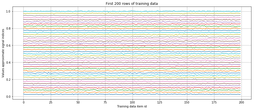
We simulate data by generating 40 different signals. Each signal has an ideal values that is characterized by its mean. For easy interpretation, we used the signals index plus one for an ideal value. So the signal indexed by zero is approximately one, the signal indexed by one about two, etc. For each data point some noise is added. The noise is drawn from a random normal distribution with zero and 0.1. All data are normalized. This is important to avoid numerical errors when computing the graph.
N = 1000000
sigma = 0.1

data = np.random.normal(size=(N,n_input))
mux = np.reshape(np.repeat(np.arange(n_input)+1,N),(N,n_input), order='F')
sigx = np.reshape(np.repeat(sigma, n_input*N), (N,n_input))
traindata = (data*sigx+mux)/float(n_input)

data = np.random.normal(size=(N,n_input))
sigx = np.reshape(np.repeat(sigma*2., n_input*N), (N,n_input))
testdata_n = (data*sigx+mux)/float(n_input)

data = np.random.poisson(size=(N,n_input))
sigx = np.reshape(np.repeat(sigma, n_input*N), (N,n_input))
testdata_p = (data*sigx+mux)/float(n_input)
plt.figure(figsize=(15,6))
plt.plot(traindata[0:200,:])
plt.grid(True)
plt.xlabel('Training data item id') ; plt.ylabel('Values approximate signal indices')
plt.title('First 200 rows of training data') ;
plt.show()
Let’s start off
Now things get interesting. Building an autoencoder is as simple as instantiating a MultilayerPerceptron object with the same number of input and output nodes in the NN graph. Additionally, we define some common activattion functions.
Training
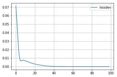
Training is just one call to the train method together with training data. We store the result of the training process, which is the progress of the loss during training. The plot below shows that loss is decreasing. That’s good because it means that the optimizer effectively manages to reduce the error. At some point the curve flattens out. That indicates that the NN converges. More precisely, the function approximated by the NN is as good in sync with the training dataset as possible given all the other parameters. Caveat: This neither means that the error is good enough for a specific application, nor that future input to the training might not lower the error even more.
Furthermore, we compute the anomaly scores of training and test data sets.
# Build autoencoder neural network graph
autoencoder = MultilayerPerceptron([n_input, n_hidden_layer, n_input], [tf.nn.relu, tf.nn.sigmoid])

# Launch the graph
lossdev = autoencoder.train(traindata)
scoretrain = autoencoder.score(traindata)
scoretest_n = autoencoder.score(testdata_n)
scoretest_p = autoencoder.score(testdata_p)

plt.plot(lossdev, label='lossdev')
#plt.plot(scoredev, label='scoredev')
plt.grid(True)
plt.legend()
...................................................................................................
Results
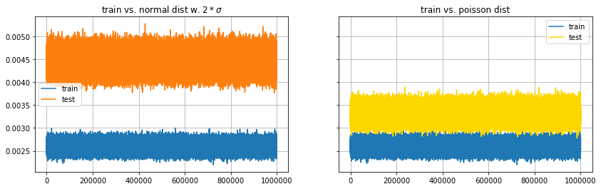
The first plot depicts low-pass filtered anomaly scores for training and test sets. The scores are in different bands. This is most likely due to the fact that the test data was generated with double the variance of the training data. The mean of the test data’s anomaly score band is around 0.0045 and its about 0.001 wide. That corresponds well with the double increase in variance.
The second chart displays the anomaly score retrieved from the Poisson distributed test set. The autoencoder separates both distribution very well. Thus, the autoencoder fulfills one basic requirement for an anomaly detector, that is to reveal data generated by different mechanisms.
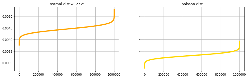
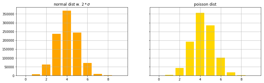
The reminder of this notebook visualizes some of the statistical properties of the anomaly scores.
f, (axn, axp) = plt.subplots(1,2, sharey=True, figsize=(14,4))
axn.plot(movingaverage(scoretrain,10), label='train')
axn.plot(movingaverage(scoretest_n,10), label='test')
axp.plot(movingaverage(scoretrain,10), label='train')
axp.plot(movingaverage(scoretest_p,10), label='test', color='gold')
axn.grid(True) ; axn.legend() ; axp.grid(True) ; axp.legend()
axn.set_title('train vs. normal dist w. $2*\sigma$')
axp.set_title('train vs. poisson dist')
<matplotlib.text.Text at 0x17764d3c8>
f, (axn, axp) = plt.subplots(1,2, sharey=True, figsize=(14,4))
axn.plot(sorted(movingaverage(scoretest_n,10)), label='test', color='orange', linewidth=4.)
axp.plot(sorted(movingaverage(scoretest_p,10)), label='test', color='gold', linewidth=4.)
axn.grid(True) ; axp.grid(True)
axn.set_title('normal dist w. $2*\sigma$') ; axp.set_title('poisson dist')
plt.show()
f, (axn, axp) = plt.subplots(1,2, sharey=True, figsize=(14,4))
histn,x = np.histogram(movingaverage(scoretest_n,10),bins=10)
histp,x = np.histogram(movingaverage(scoretest_p,10),bins=10)
axn.bar(np.arange(len(histn)), histn, color='orange')
axp.bar(np.arange(len(histp)), histp, color='gold')
axn.grid(True) ; axp.grid(True)
axn.set_title('normal dist w. $2*\sigma$') ; axp.set_title('poisson dist')
plt.show()
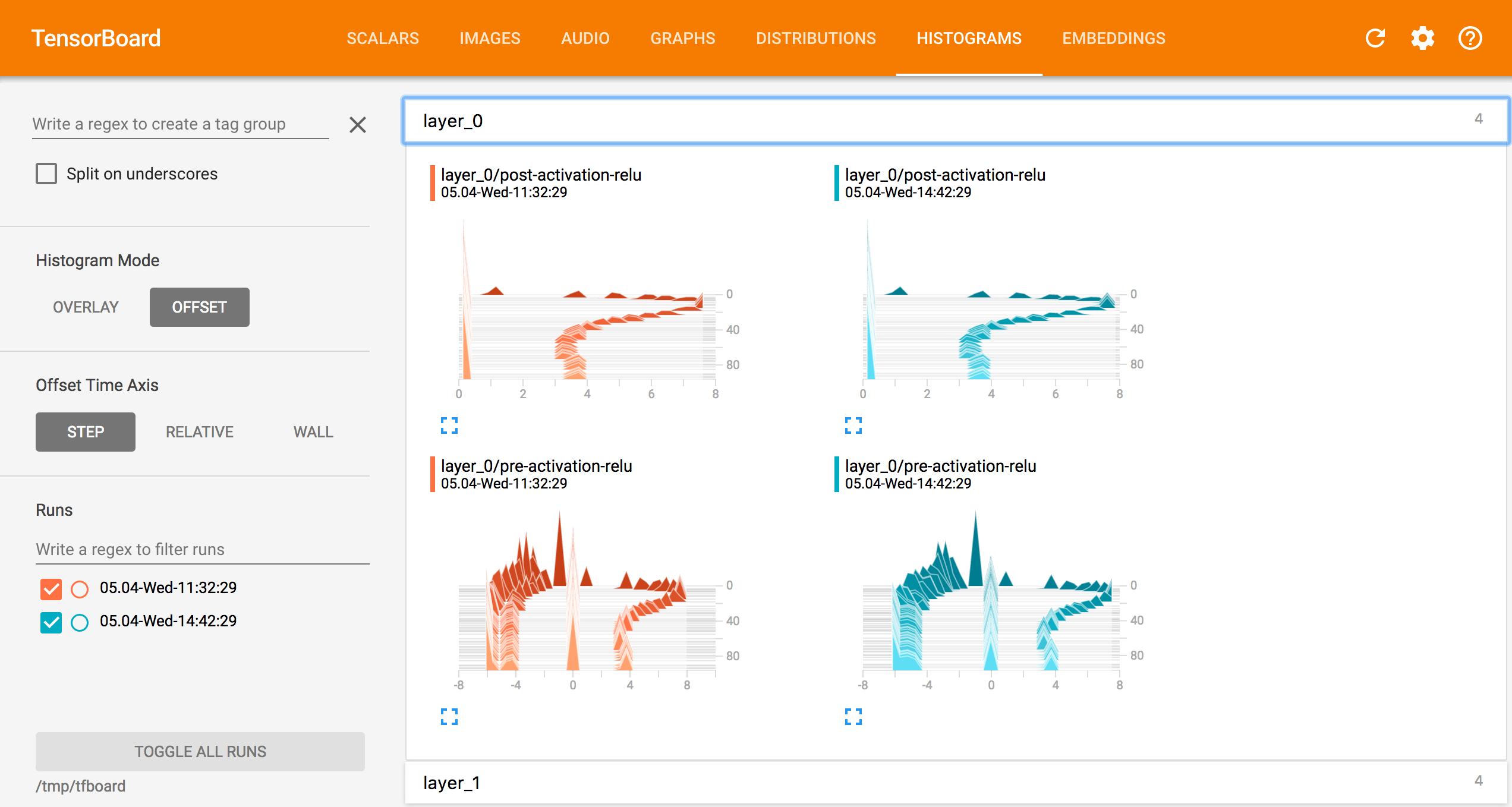
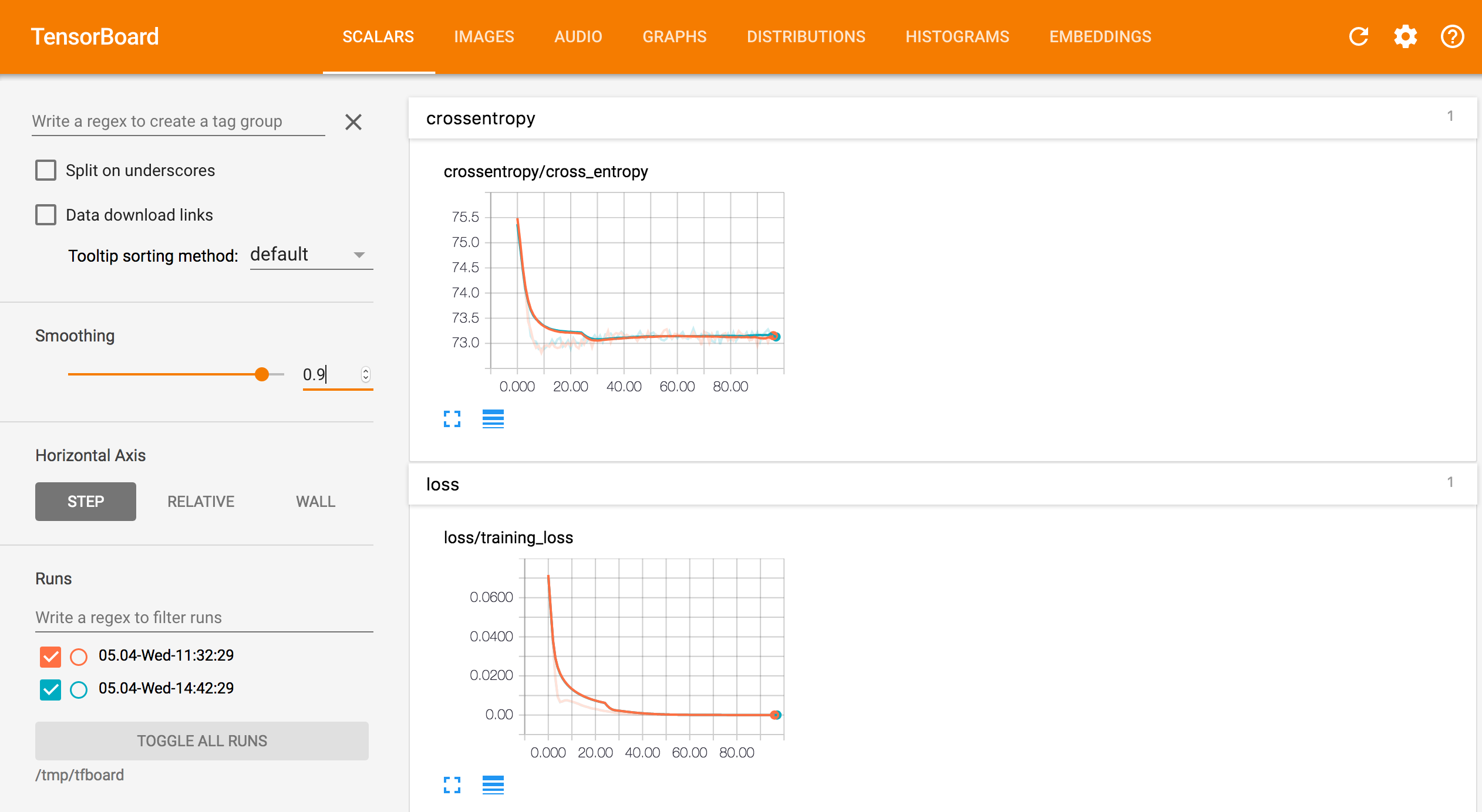
Appendix -Tensorboard Screenshots
Graph
Learning progress
Perceptrons